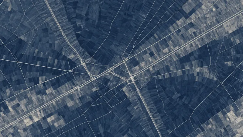
A 3-meter C-band SAR pass can preserve a pipeline corridor's surface signal under cloud, while a submeter optical pass from the same week may contain no usable ground pixels.
That contrast is the practical reason to combine the two sources for pipeline right-of-way inspection. Synthetic aperture radar records the interaction between microwave energy and the ground, vegetation, structures, and moisture conditions. Optical imagery records reflected energy in visible and infrared bands, giving an analyst the color and texture needed to interpret what changed. One source provides continuity through weather and darkness. The other provides context that is much easier to read.
Combining them is harder than placing two images in adjacent map panels. The sensors use different geometries, resolutions, noise models, acquisition schedules, and definitions of what constitutes a meaningful change. A useful inspection pipeline has to preserve those differences long enough to model them, then align the outputs so that an analyst can evaluate a common location and time window.
What Each Sensor Contributes to a ROW Inspection
Optical imagery is usually the first layer people reach for because it resembles the visual scene. Multispectral bands can support vegetation analysis, including NDVI for identifying changes in plant vigor or cleared ground. Panchromatic imagery can provide finer spatial detail, and pansharpening can combine that detail with multispectral color information. For a right-of-way, those products help distinguish bare soil, mowed vegetation, standing water, access roads, construction material, and nearby land use.
Optical data also has familiar failure modes. Cloud cover can remove an entire observation opportunity, particularly in humid or storm-prone regions. Haze reduces contrast. Shadows from terrain or infrastructure can obscure the feature of interest. A scene can have a nominally good quality score and still be unhelpful over the particular section of ROW that matters.
SAR does not depend on sunlight and is less affected by cloud cover. A C-band product can respond to surface roughness, moisture, vegetation structure, and the orientation of objects relative to the radar look angle. L-band has a longer wavelength and can interact differently with vegetation and the ground. Polarizations such as VV and VH provide additional information about scattering behavior, although their value depends on the sensor, collection geometry, and scene conditions.
For monitoring, we may also examine backscatter intensity and interferometric coherence. A change in intensity can indicate altered surface or vegetation conditions. A reduction in coherence can indicate that the scene has changed between acquisitions, but it does not identify the cause on its own. Soil moisture, agricultural activity, wind, vegetation movement, and temporal decorrelation can all affect the signal.
That last point is important. SAR is not a direct substitute for a photograph, and a bright or dark radar response is not a violation report. It is evidence that needs to be interpreted with geometry, history, and other observations.
The Registration Problem Comes Before the Fusion Model
When we built the pipeline ingestion layer, the first recurring problem was not model selection. It was spatial and temporal registration. A SAR product may be delivered in a projected coordinate system with a particular ground-range convention. Optical imagery may be orthorectified against a different elevation model. Their pixels can appear aligned at a broad map scale while being offset enough to move a narrow linear feature across several cells.
For a pipeline corridor, that error matters. A buried line, access track, drainage channel, or fence can be only a few meters wide. If the SAR and optical layers are not co-registered, a model may learn that a neighboring feature is the source of a response. We treat geolocation quality, acquisition geometry, and pixel spacing as inputs to the processing graph rather than metadata to ignore after download.
The temporal relationship is just as important. A SAR scene collected after heavy rain and an optical scene collected during a dry period are not observing the same surface state. A recently mowed ROW may look like vegetation loss in optical imagery while producing a different radar response because the exposed soil is wet. A construction vehicle can create a temporary roughness change that disappears before the next optical pass.
Our normal sequence is to normalize each source independently, preserve the original measurements, and create derived features only after the spatial and temporal relationships are explicit. For SAR, that can include calibrated backscatter, terrain correction, speckle filtering, incidence angle, look direction, and polarization channels. For optical data, it can include cloud and shadow masks, surface reflectance when available, band quality flags, multispectral indices, and a record of whether pixel fusion or pansharpening was applied.
Speckle filtering deserves restraint. A filter can make a SAR image easier to inspect, but aggressive smoothing can remove the small-scale variation that distinguishes a disturbed strip from its surroundings. We generally keep a filtered representation for visual and model features while retaining the calibrated, unfiltered signal for audit and comparison.
A Synthetic ROW Scenario
Consider a 42-kilometer section of pipeline ROW crossing wetlands, pasture, and a low-density residential area. The inspection team receives a cloudy optical scene from the first collection window. The corridor is visible in a few gaps, but most of the central section is masked. Two days later, a commercial C-band SAR provider collects a 3-meter scene with VV and VH channels. The acquisition has a different look angle from the prior SAR scene, and the area received significant rain between observations.
The initial temptation is to run change detection on the radar pair and use the optical image only where it is clear. That approach produces several plausible but ambiguous candidates. A recently graded access track has a strong intensity change. A wet drainage area also changes. A patch of wind-disturbed reeds loses coherence. None of those responses identifies a pipeline threat by itself.
We would first construct a corridor-centered analysis grid, with a buffer wide enough to capture the ROW, access points, drainage, and adjacent land use. The grid stores each acquisition's footprint, timestamp, incidence angle, polarization, cloud mask, and estimated data quality. It also stores the distance and orientation of candidate changes relative to the ROW centerline. That relational context is often more useful than a raw anomaly score.
Where the optical image is valid, multispectral values and NDVI change can help separate bare soil from vegetation stress. A candidate with a new linear shape, a sustained optical signal, and a corresponding SAR response deserves more attention than a single-channel radar fluctuation. Where optical coverage is absent, SAR can preserve the candidate in the inspection queue, but the system should label the evidence as radar-only rather than imply that the same level of interpretation is available.
For a wetland segment, we might compare the candidate against several prior SAR acquisitions rather than a single baseline. A persistent change in backscatter or coherence is more informative than a one-pass deviation following rain. For the residential segment, optical context may be decisive because roofs, vehicles, tree shadows, and fences can create radar responses that are difficult to interpret from backscatter alone.
The output is not a single fused image. It is a spatial view containing source layers, derived features, acquisition conditions, candidate geometries, and an explanation of which observations support each candidate. That structure lets an analyst inspect the evidence without losing the distinctions between a measurement and an inference.
Fusion Strategies and Their Tradeoffs
There are several reasonable points at which to combine SAR and optical data. Pixel-level fusion is the most direct. Resampled bands and radar channels are stacked into one tensor, often after pansharpening or another pixel fusion step. This can work when the sources are closely matched in time, accurately registered, and sampled at compatible resolutions. It becomes fragile when one source has cloud gaps, different ground sampling distance, or a substantial acquisition-time difference.
Feature-level fusion is more flexible. Each modality gets its own preprocessing and encoder, and the resulting features are combined before classification or ranking. This lets the SAR branch model speckle, polarization, and incidence angle while the optical branch handles spectral relationships and cloud masks. The model can also receive missing-data indicators instead of treating an absent optical pixel as a valid zero.
Decision-level fusion combines independent outputs, such as an optical vegetation-change score and a SAR disturbance score. It is easier to audit and deploy incrementally, but it can hide conflicts between the sources. A weighted average may produce a confident-looking result when the two inputs disagree for a meaningful reason. We prefer to retain source-specific scores and expose the disagreement as part of the result.
In practice, the best architecture is often a hybrid. Source-specific preprocessing produces comparable spatial features. A fusion layer combines them where coverage and quality support it. A final ranking step includes acquisition metadata, temporal persistence, distance to the ROW, and known confounders. The model's output should include provenance, not just a probability.
Spatial resolution also limits what fusion can accomplish. A 3-meter SAR product and a submeter optical product do not become submeter radar observations when stacked together. Resampling can align grids, but it cannot create detail that the coarser sensor did not collect. The model may use fine optical structure to contextualize a broader radar response, but the distinction between those information scales needs to remain visible.
When Fusion Adds More Complexity Than Value
Fusion is not automatically the right choice for every inspection interval. If a corridor sits in a dry region with consistently clear skies, frequent high-quality optical coverage may answer the operational question with less processing and lower cost. If the task is limited to broad vegetation condition, the additional calibration and geometry handling required for SAR may not improve the decision.
The same applies when revisit intervals do not match the inspection cadence. Commercial SAR providers now offer products around 3 meters with daily revisit in some orbits, but availability depends on location, collection plan, look angle, and ordering constraints. A nominal revisit number does not guarantee a usable observation over the exact corridor on the required day. Adding SAR to a workflow without a dependable acquisition plan creates another layer of missing data to manage.
There is also a human cost. Analysts need to understand why a radar candidate appears, how weather may have affected it, and when an optical and SAR observation should not be compared directly. If the fused result collapses those distinctions into one unexplained alert, it can increase review time rather than reduce it.
The limitation worth naming directly is that SAR and optical fusion cannot resolve an ambiguous physical cause when the available observations do not contain enough evidence. It cannot identify an unauthorized excavation from a single coherence loss, infer buried pipeline condition from surface imagery alone, or compensate for a missing baseline. Fusion improves coverage and context. It does not turn indirect surface measurements into direct inspection of subsurface assets.
What We Put in the Spatial View
At Larx, we think about this workflow as a decision-intelligence problem rather than an image-display problem. The useful unit is not an isolated scene. It is a location with a time series, multiple sensor observations, quality information, derived measurements, and a review state.
That means the interface should allow an analyst to compare a SAR intensity layer, coherence change, optical bands, NDVI, and source masks without navigating separate systems. It should also show when a candidate is supported by both modalities, when it is supported by only one, and when the observations conflict. A candidate's confidence should be conditional on the data that actually exists.
For machine learning, this representation helps with training and evaluation. Labels can be tied to corridor segments and acquisition windows instead of copied across every pixel in an image. Negative examples can include known confounders such as wet soil, mowing, shadows, and temporary equipment. Model performance can then be measured by inspection workload and candidate quality, not only by pixel-level accuracy.
The practical friction remains in the handoffs: acquiring the right scene, checking its geometry, masking invalid pixels, aligning timestamps, preserving source provenance, and explaining disagreement between sensors. Before the imagery combination helps an inspection program, those ordinary processing details have to be correct at the same corridor location and the same observation window.