Setting the Baseline Is Harder Than Running the Change Detection
Stormwater change detection fails most often because the baseline image represents a different season, moisture condition, or acquisition geometry than the image being compared. The subtraction is easy. Selecting observations that make the subtraction meaningful is the engineering work.
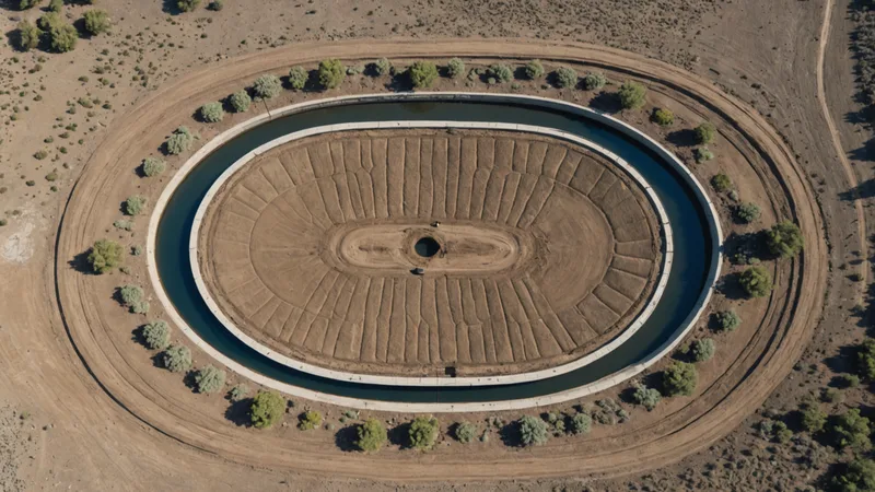
A BMP site can look materially different in optical imagery without any structural change. A detention basin may be dry in one acquisition and holding water in the next. Grass can move from dormant brown to dense green between two otherwise comparable images. A cloud shadow can lower reflectance across half a site. Even when the ground has not changed, the pixel values have.
For stormwater monitoring, the useful question is not simply whether two images differ. It is whether the observed difference is consistent with a site condition that deserves attention: a breached berm, altered outfall, exposed soil, removed vegetation, expanding bare area, standing water that persists beyond the expected period, or construction activity near a protected feature.
What a Useful Baseline Contains
A single image from six months ago is a starting point, not necessarily a baseline. For each BMP, I want a time window and an observation set that describe normal variation at that location. In practice, that often means collecting several cloud-screened images over 12 to 24 months, then building seasonal composites rather than selecting one visually attractive scene.
The appropriate number depends on revisit frequency, cloud conditions, site size, and the decision being supported. Three usable observations in a season may be enough for a simple triage workflow. A site with frequent vegetation cycles, intermittent ponding, or repeated construction activity benefits from more. The objective is not to create a perfect historical archive. It is to estimate the range of expected surface conditions well enough that an alert represents an unusual departure.
Temporal composites help separate persistent site characteristics from acquisition noise. A median composite can suppress isolated artifacts and small transient features. A percentile composite can preserve information about wetness or exposed surface conditions when that range matters. The comparison window also needs to be operationally relevant. If a team is prioritizing visits before an inspection cycle, a recent 30 to 90 day reference may be more useful than a broad annual average.
Image registration is another prerequisite. A one or two pixel shift along a basin edge can appear as a ring of change, particularly when water, gravel, and vegetation meet at a sharp boundary. The imagery must be aligned consistently, and the analysis should use a site buffer that distinguishes the BMP footprint from nearby roads, parcels, and unrelated grading.
Seasonal Variation Is a False Positive Factory
Vegetation phenology creates some of the most persistent false positives in optical change detection. A grassed swale in April and the same swale in August can have different normalized difference vegetation index, or NDVI, values across nearly every pixel. That does not mean the swale has failed. It means the model has observed a seasonal cycle.
NDVI is useful for detecting vegetation loss, but it should not be treated as a universal condition score. Other combinations can help characterize the change. The normalized difference water index can provide evidence of altered surface water. Shortwave infrared bands can help distinguish moisture and exposed soil. Red edge bands can add sensitivity to vegetation stress where the source imagery supports them. Bare soil indices and simple band ratios can identify newly exposed surfaces, but they remain sensitive to illumination, soil type, and moisture.
The practical approach is to compare like with like. A spring observation should be compared against other spring observations where possible. Seasonal thresholds should be learned separately, and an alert should require more than a single index crossing a fixed value. For example, a candidate vegetation-loss area becomes more credible when NDVI declines, a bare-soil indicator rises, and the changed pixels form a coherent patch within the BMP boundary.
Spatial shape matters. A diffuse change covering the entire site may indicate seasonal or atmospheric effects. A narrow linear feature along an embankment, a new polygon around an outfall, or a growing patch immediately downstream deserves a different score. Thresholds should therefore combine spectral magnitude, persistence, connected area, and location relative to mapped site features.
Clouds, Shadows, and the Missing Observation Problem
Cloud contamination is not solved by simply dropping images with a high scene-level cloud percentage. A scene listed as 10 percent cloudy can still place a cloud or cloud shadow directly over the basin. Conversely, a scene with more cloud cover may contain a clear and useful site footprint. Quality screening has to operate at the site or tile level, with cloud and shadow masks applied before statistics are calculated.
For most optical workflows, I prefer cloud-free mosaic windows over a single acquisition. A 15 to 30 day window can provide enough clear pixels to construct a representative observation while preserving temporal meaning. Longer windows improve coverage but can blur a real event. If a contractor removes sediment or repairs an outfall during that period, the composite may describe neither the pre-work nor the post-work condition accurately.
Persistent cloud cover creates a second problem: missingness can become geographically biased. Coastal and mountainous regions may have fewer usable optical observations precisely when monitoring is most needed. Synthetic aperture radar, or SAR, provides a fallback because it can collect through clouds and at night. Radar backscatter responds to surface roughness, moisture, and structure, so it is not a drop-in replacement for optical indices. It needs its own baseline, normalization, and interpretation rules.
Optical and SAR alerts are strongest when treated as different evidence streams. A radar anomaly after heavy rain may indicate changed moisture or roughness, but it is not by itself proof of a damaged BMP. A persistent anomaly across multiple radar observations, supported by optical evidence when a clear image arrives, is more useful for field prioritization than either signal alone.
From Pixel Difference to Inspection Priority
A change map is not yet a workflow. Stormwater teams need an alert that explains why a site was selected, how much of the site changed, whether the change persisted, and what evidence supports the decision.
Consider a consultant managing 86 BMP sites across three mid-Atlantic counties before a permit inspection cycle. The team cannot visit every site in the same week. A useful process would first remove sites with insufficient clear coverage, then compare each site against season-matched composites. Sites with a stable spectral profile remain in the routine queue. Sites with a new bare-surface polygon near an outfall, a persistent water anomaly, or a change along an embankment move into a review queue. The consultant can then inspect the imagery, check available sensor readings, and schedule physical visits for the highest-confidence cases.
The ranking should preserve uncertainty rather than hide it. An alert with 40 percent valid pixels, weak seasonal separation, and one anomalous image is different from an alert with 95 percent valid pixels, three consecutive observations, and agreement between optical and sensor data. Those distinctions can be represented with confidence fields, not just a red or green label.
Sensor integration adds temporal context. A water-level sensor, turbidity reading, precipitation record, or flow measurement can help explain why imagery changed. If a ponding anomaly appears after a recorded storm and disappears in the next observation, it may be expected behavior. If the surface signal persists while sensor conditions return to normal, the event deserves a different review. The sensor does not eliminate the need for imagery interpretation, but it can reduce avoidable field visits.
This is not a claim that satellite imagery replaces permit-required site visits. It is a claim about which sites actually need one before the inspection window closes. The point is prioritization, with enough traceable evidence that a reviewer can understand why a site entered the queue.
What Change Detection Does Not Catch Reliably
Surface change is not the same as infrastructure condition. Satellite imagery will not reliably identify subsurface damage, internal erosion, or a compromised pipe that has not altered the visible surface. Sediment accumulation can remain below the spatial and spectral sensitivity of the imagery, particularly when the surface still resembles surrounding soil or vegetation.
Heavy canopy cover creates another hard boundary. A failure beneath trees may be invisible in optical imagery, and radar returns can be difficult to interpret where branches, trunks, and wet ground contribute to the signal. Small features may also fall below the effective resolution of the source imagery. Anything requiring a physical measurement, such as depth, slope, structural integrity, or material thickness, remains a field task.
These limitations should shape the alert design. A system should label a result as a surface-change indication, not as a compliance determination or a confirmed failure. That distinction matters when imagery is used alongside inspection records, rainfall history, work orders, and sensor observations.
Where Larx Fits in the Workflow
Larx handles the multitemporal imagery pipeline and brings the resulting change signals into a unified spatial view with sensor data for infrastructure and environmental teams. For stormwater monitoring, that means baseline images, seasonal comparison logic, configurable thresholds, and automated alerts can be managed as part of the same site workflow rather than as disconnected image exports and spreadsheets.
The technical value is in preserving the context around an alert. A reviewer can see the comparison interval, valid-pixel coverage, detected change area, relevant spectral evidence, and associated sensor observations before deciding whether to assign a field visit. That supports a narrower operational goal: filtering expected seasonal variation and acquisition noise well enough that the remaining queue is manageable.
When the workflow is working, most sites produce no drama. They remain in the routine queue, while a short list of persistent, spatially coherent changes receives human review and a scheduled visit.