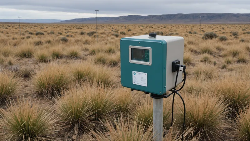
The stormwater detention site in the Chesapeake watershed had been reporting consistent dissolved oxygen levels for eleven weeks. Then a satellite-derived change detection flag appeared near the basin outlet. The imagery showed a change in surface moisture and vegetation stress that did not fit the sensor record. Nearby conductivity readings had also shifted, although not enough to trigger the program's existing alert threshold.
The first assumption was that the imagery was wrong. The second was that the basin had experienced an unrecorded discharge or maintenance event. When the monitoring team compared the full record, a quieter explanation emerged: the dissolved oxygen probe had been drifting upward by a small amount each day. It still produced plausible values. It still followed the expected daily pattern. It was simply becoming less accurate.
That is the difficult character of sensor drift. A failed instrument is usually easier to find than a biased one. A dead thermistor, a flat-lined tipping-bucket rain gauge, or a conductivity probe returning impossible values can be isolated quickly. Drift does not announce itself. It can remain inside the range of reasonable readings while gradually weakening the decisions built on top of those readings.
The dangerous sensor is the one that still looks plausible
Environmental monitoring programs are often organized around individual instruments. Each sensor has a location, a maintenance schedule, a calibration record, and a time series. Those are necessary controls, but they can create a narrow view of performance. A reading may be technically valid as a data point while being misleading in relation to the surrounding site.
Consider a pH sensor installed downstream of a stormwater best management practice. A small upward bias might not stand out in a daily report, especially if rainfall, temperature, and flow conditions vary. If the sensor reads 2 degrees high every day, it may look fine in isolation. Against a spatial baseline that includes satellite change data and adjacent sensors, the drift can become visible within days.
The same problem appears in other forms:
- A turbidity probe becomes partially fouled and responds more slowly after rainfall.
- A dissolved oxygen instrument reports a stable pattern while its membrane or optical cap is degrading.
- A conductivity sensor develops a bias after repeated exposure to sediment or changing salinity.
- A tipping-bucket rain gauge undercounts during intense events because of debris, leveling problems, or mechanical wear.
None of these conditions necessarily produces an absurd value. The record can retain enough regularity to pass a basic quality check. The warning often appears only when the reading is compared with something outside the instrument's own history.
What spatial cross-validation adds
Cross-validation is not the same as assuming that every nearby data source should agree. Environmental conditions vary in space, and sensors positioned only a short distance apart can measure different water, soil, or microclimate conditions. The purpose is to examine whether independent observations support the same interpretation.
In the detention basin scenario, the team assembled several reference layers: readings from an upstream conductivity sensor, rainfall totals from a nearby gauge, recent inspection notes, thermal imagery, and satellite-derived changes in vegetation and surface moisture. None of those sources could directly measure dissolved oxygen at the probe location. Together, however, they described a site that was changing in ways the dissolved oxygen record did not reflect.
The comparison raised useful questions:
- Did the sensor change at the same time as rainfall, flow, or temperature conditions?
- Did adjacent instruments respond to the same event?
- Did the spatial pattern around the basin support the reported value?
- Was the sensor's relationship with other measurements stable over time?
This approach is especially useful for monitoring programs connected to municipal separate storm sewer system, or MS4, permits. Permit obligations differ by state and by jurisdiction, but programs commonly involve outfall inspections, stormwater BMP evaluations, recordkeeping, and follow-up when conditions indicate a potential issue. A spatial record does not replace those requirements. It can help a coordinator decide where a field check or resampling effort deserves attention.
A plausible failure pattern in a stormwater program
Imagine a mid-Atlantic consulting team monitoring a detention basin and two downstream outfalls for a municipal client. The program includes monthly field visits, continuous conductivity and dissolved oxygen measurements, a tipping-bucket rain gauge, and periodic water-quality sampling. The basin was designed to reduce pollutant loads before discharge, so changes in residence time, vegetation, or standing water could affect how the BMP performs.
For most of the season, the dissolved oxygen record followed a familiar pattern. Values rose during daylight hours and declined overnight. No alert threshold was crossed. The field technician's visual notes described ordinary conditions, with no obvious fish stress, odor, or discoloration.
After a sequence of storms, satellite imagery showed a persistent wet area along one side of the basin and a change in vegetation near the outlet. Conductivity at the downstream sensor also increased after rainfall and stayed elevated longer than expected. The dissolved oxygen record, by contrast, continued its previous smooth cycle.
The team inspected the probe and found fouling that had not yet caused a complete failure. A calibration check confirmed a bias. The earlier data could not simply be discarded, because some of it might still have been useful after correction. But it could no longer be treated as an independent account of basin conditions.
The operational lesson was not that satellite imagery had diagnosed the probe. It had not. The value came from the contradiction. The spatial record made it harder to accept a clean sensor trace without asking what else was happening at the site.
Cross-validation has failure modes too
Spatial cross-validation can catch a blind spot, but it can also create false concern. Satellite observations may be affected by cloud cover, viewing angle, seasonal vegetation changes, or a resolution that blends several land-cover conditions together. An adjacent sensor may be poorly maintained as well. A rainfall gauge may be technically sound but located far enough away to miss a localized storm.
There is also a timing problem. Imagery may be collected hours or days apart, while an in situ instrument records every few minutes. Comparing the two requires care about acquisition time, lag, and the physical process being observed. A vegetation response may reflect accumulated moisture over several days, not the condition at the exact moment of a sensor reading.
For that reason, a disagreement should be treated as a reason to investigate, not as proof that one source is correct. We prefer to ask whether several independent signals point in the same direction and whether the proposed explanation fits the site's physical behavior. That may lead to a field inspection, a grab sample, a calibration check, or a review of recent maintenance and weather records.
What we noticed when building the Larx platform is that the difficult part is not placing every source on a map. The difficult part is preserving enough context to understand why sources disagree. A sensor alert without recent rainfall, asset location, inspection history, or nearby observations leaves too much interpretation to a later handoff.
What the monitoring team still has to do
Spatial cross-validation is not a substitute for calibration, cleaning, inspection, or professional judgment. It cannot determine the condition of a probe that was never installed correctly. It cannot recover a measurement that was not collected. It cannot establish regulatory compliance on its own, and it cannot distinguish every environmental change from an instrument problem without field evidence.
The monitoring program still needs a defined response path. Someone must decide how much disagreement warrants a site visit, how suspect data will be flagged, when a sensor will be removed from service, and how corrected values will be documented. Those decisions should be made before a questionable record becomes part of a permit report or a maintenance recommendation.
It also helps to design the baseline before the first failure. Record the expected relationships among rainfall, water level, conductivity, turbidity, temperature, and dissolved oxygen. Note which comparisons are meaningful and which are not. Establish what a normal delay looks like after a storm. A baseline built only after an anomaly appears will be harder to interpret.
The drift problem is not primarily a sensor calibration problem. It is a program design problem: how do you build a record that can catch its own errors before they propagate? The answer is not to distrust every instrument or to treat a map as an oracle. It is to give each important measurement enough environmental context that a quiet contradiction can become visible while there is still time to investigate it.